Loss Landscapes

Visualizing the Loss Landscape

The loss landscape graphically represents the model’s loss function, a measure of how well the model can make predictions on a given dataset. Previous work has shown that structure of the loss landscape foretells the generalizability and robustness on a model solution (Keskar et al.). Furthermore, recent optimization methods leverage local loss information to traverse the loss landscape and lead to drastic training improvements (Foret et al). Most papers use loss visualization to validate model performance and provide comparison between solutions. In contrast, here we describe methods and heuristics for analyzing the loss landscape with the intention to improve model architecture, adjust training hyperparameters, and gain insight into the training process of large models.

A Deeper Background Into Loss

In deep learning, the loss function used in the loss landscape measures the difference between the model’s predicted output and the true output. Loss metrics, such as mean squared error or cross-entropy loss, calculate the difference in ways important to the prediction power of the problem. Then, gradient descent algorithms used to train the model adjusts the model’s parameters in order to minimize this loss function, ultimately leading to a model that is able to make accurate predictions. Importantly, by minimizing loss through the optimization process, we improve the model’s ability to make accurate predictions on unseen data.

Deep learning differs from traditional optimization in that the process for obtaining a minima matters more than the actual value of the minima achieved. For example, the figure below depicts a vision transformer trained with two different optimization techniques. Despite one model having substantially lower loss and higher training accuracy, its test accuracy is 10% lower.

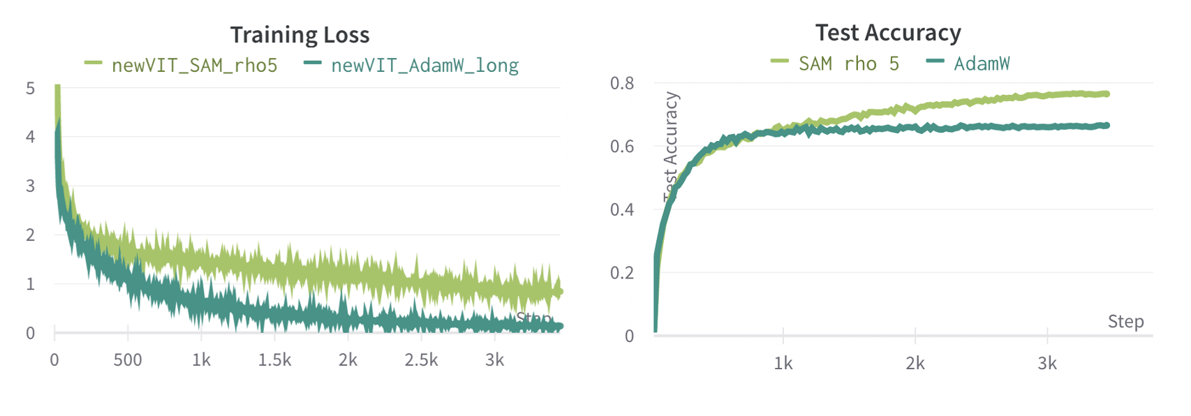
This problem initially appears to be due to overfitting. Classical machine learning describes overfitting as the point in training where the model begins to have high training performance by learning features specific to the training set. Overfitting is typically overcome by adding regularization.

Though the models above contain far sufficient parameters to overfit, they cannot be overcome by regularization techniques alone. As seen below, increasing the regularization (as either weight decay or Gaussian noise) did not improve the model test performance.

Rather, the model was improved using local loss information to smooth the loss landscape in a process called Sharpness Aware Minimization (SAM). Training with insight to the loss landscape provides many approaches to improving deep learning models, though it is critical to develop a fundamental understanding of loss landscapes and SAM.

Loss Landscapes

After training a model, one can visualize the loss landscape by using various techniques that reduce the high dimensionality of the model’s parameter space and the data space to a two-dimensional surface. This is known as a loss landscape. The loss landscape graphically represents how the model’s loss function changes as the model parameters change. The graph is centered on the optimal model parameters, resulting distinctive “valley” shape, with larger loss values as the parameters are shifted away from the optimal values. The shift away from the optimal parameters can be determined through many different traversal strategies, but in any case, the resulting plot is a dimensional reduction of the true parameter space of the model. Thus, examining the loss landscape’s width, smoothness, and shape provides meaningful insight into model performance in a simplified representation of the true problem defined by the data.

Previous work has shown that structure of the loss landscape foretells the generalizability and robustness on a model solution (Keskar et al.). Keskar et al explores how optimizing CNNs on small batches of data (e.g. stochastic gradient descent) vs large batches of data affect the loss landscape of models. They find that small-batch training results in loss landscapes that have a minima with a wider opening at the top, resulting in more generalizable models

More recent research has also investigated how loss landscapes can improve model training. By developing a more generalizable model early in training, the final solution reached will both be more generalizable as well as more powerful. Work (Foret et al) has found great success designing optimizers around finding smoother areas of the loss landscape. Sharpness-Aware Minimization, or SAM, minimizes both loss and loss sharpness. This directly causes the loss landscape to be smoother while training, and the results are impressive! A ResNet-101 model trained on ImageNet using SAM had a 3.3% error decrease compared to a equivalent model without SAM. Similarly our Visual Transformer model showed a 10% improvement on ImageNet-100 using SAM as seen in the image below.

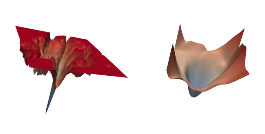Image from Foret et al Depicting loss landscapes before (left) and after (right) training with SAM

Sharpness Aware Minimization (SAM)

Sharpness Aware Minimization (SAM) analyzes the geometry of the parameter space induced by the symmetries of deep learning models, allowing for the identification of regions of the loss landscape where the minima are flatter. This information can be used to guide the training process and improve the performance of the model. SAM does not just identify when a good solution is reached, but forces the model in directions with smoother loss landscapes.

To gain an intuition on how SAM works, SAM directs the model training by reparameterizing the loss function. Let $f(x)$ be a function with parameters $\theta$, and let $g(\theta)$ be a reparametrization of $f(x)$. The relationship between $f(x)$ and $g(\theta)$ is given by $g(\theta) = f(x(\theta))$

The geometry of the parameter space can be changed by choosing a different reparameterizing $g(\theta)$, resulting in a new set of parameters $\theta’$ for the function $f(x)$. SAM defines the reparameterization such that the loss computed from which to step from is derived from a local maximum. The significance of this reparametrization is best described visually.

Let’s say our model wandered into a sharp minima, we start by computing the gradient as usual, which would typically lead us to oscillate in the current minima (even with momentum).

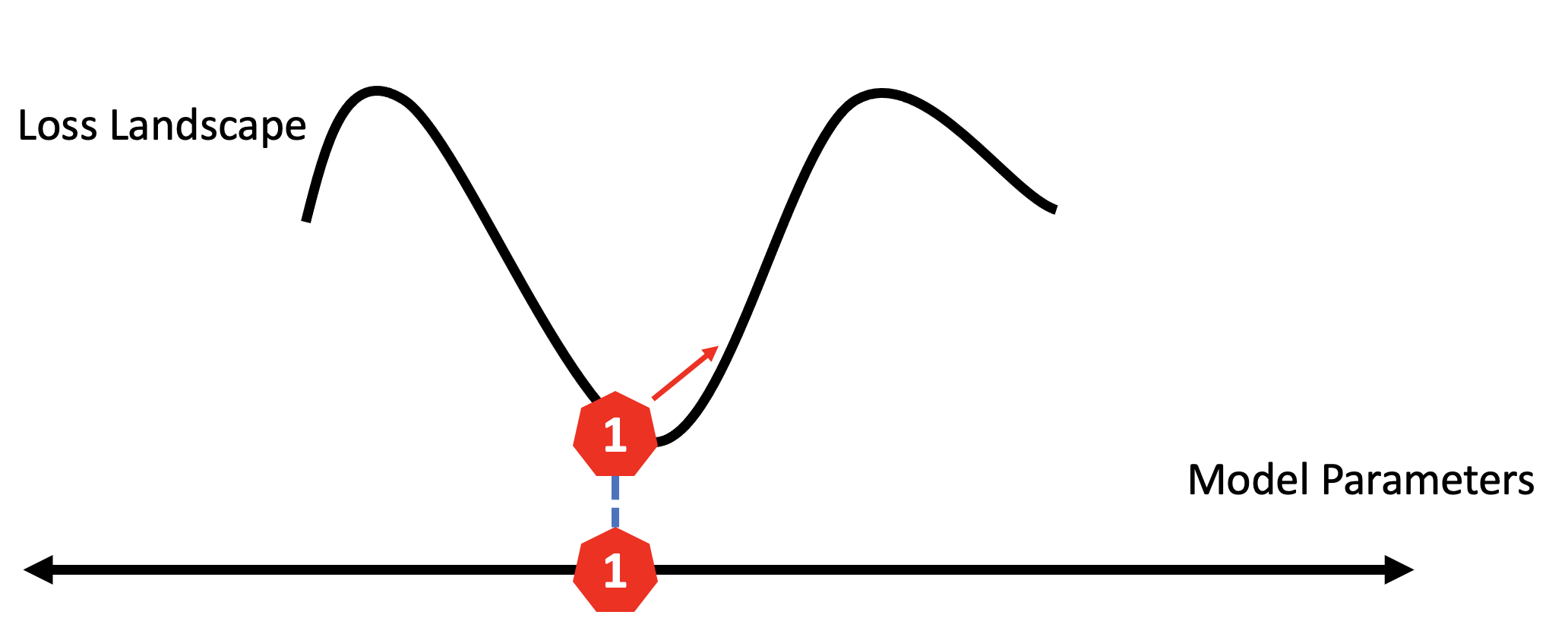
So, we then move the opposite direction, scaled by a factor called rho.

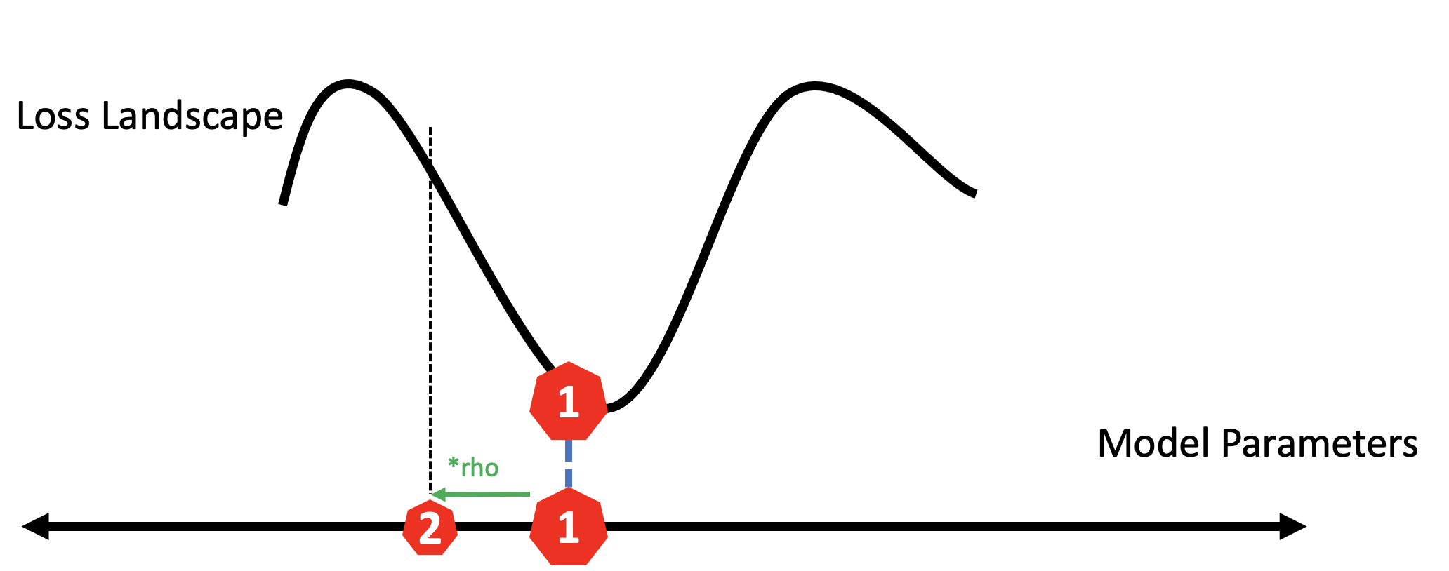
Last, we use the gradient calculated at the second location to step from our original location. This effectively uses the sharpness of the surrounding landscape to force it to new areas.

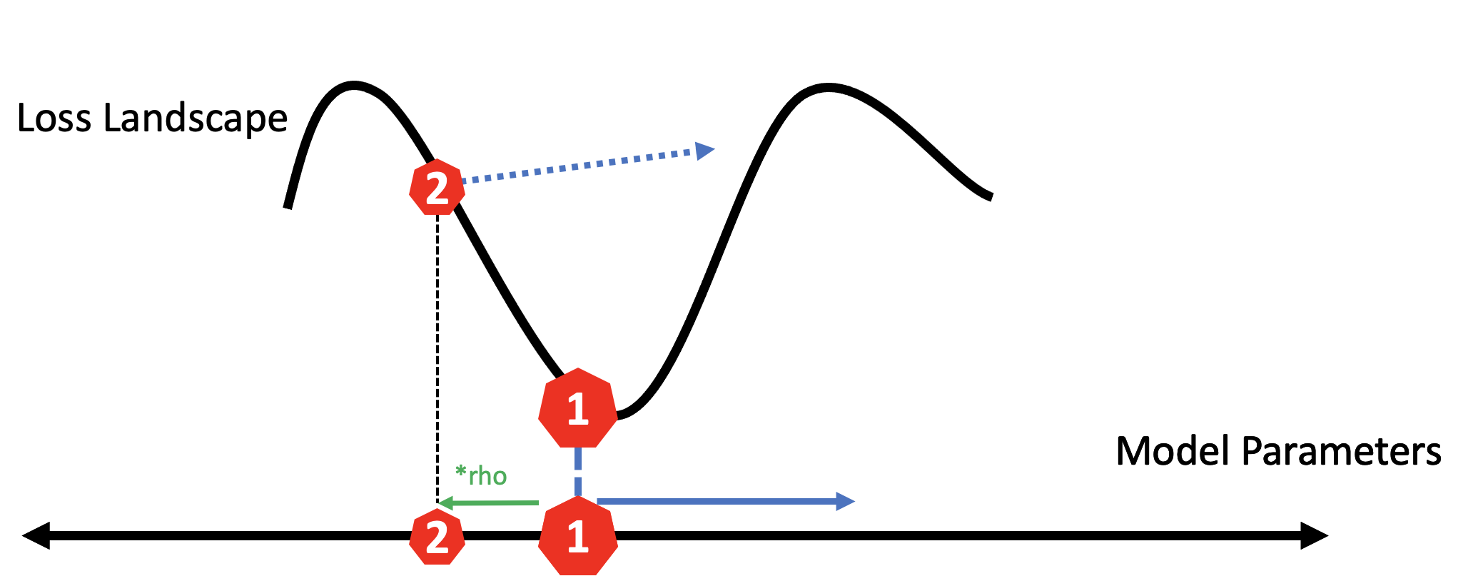
Thus, by changing the geometry of the parameter space to smooth out local minima, the model more easily identifies new regions of the loss landscape that may be more generalizable and higher performing.

Heuristics for Loss Analysis

The loss landscape graphically represents the model’s loss as a function of its parameters, which can provide insight into the training process of the model and its final test performance. The loss landscape is typically visualized as a one or two-dimensional plot, an approximation of the true high-dimensional function landscape. Thus, the loss landscape only represents a small slice of the full function space, with the dimensions and axes of the plot being determined by the specific parameters that are being visualized.

Since the loss landscape selects only a slice of the true function space, it is essential to understand the various techniques for slicing as well as heuristics for improving loss landscape reliability and interpretability. As seen in the example below, even modifications to the distance to traverse can lead to large, unintuitive changes in the loss landscape visualization. Here, we’d expect the loss landscape traversed over a 2x2 traversal grid would encompass an identical 1x1 traversal grid within the graph. Unintuitively, we see that changing the size of the traversal grid leads to a new slice and exploration that is substantially smoother.

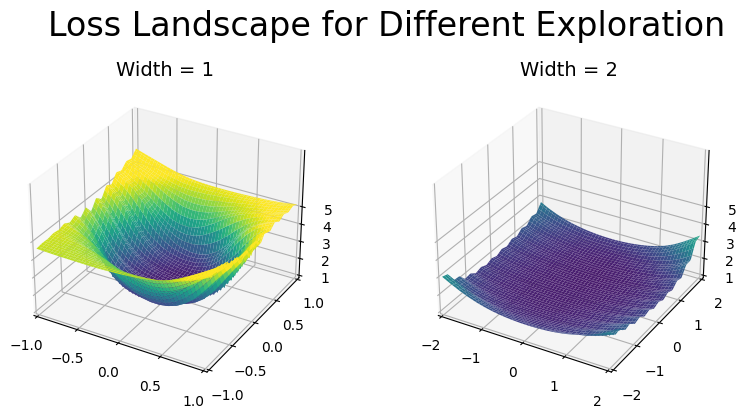
Despite this limitation, the loss landscape can still be a useful tool for understanding how the model is training and identifying potential problems or issues with the optimization process. For example, wide exploration techniques with large batch sizes may be used to evaluate data augmentation techniques. A smoothly loss landscape likely indicates that the dataset is well patched and continuous. In contrast, narrow loss exploration techniques provides insight into hyperparameterization, evaluating how fast a model is converging and to what type of solution.

To identify loss landscape plot strategies that best reveal characteristics of interest, it is important to first identify a test case and as base model. We started with the base optimizer, AdamW, and a Vision Transformer. After initial tuning, develop a loss plot strategy that reflects an average case. A single plot by itself can not be used to gain information, rather provide a base condition. By generating a plot representing an average case (a relatively smooth, but variable loss landscape), the test case can then be evaluated using the same strategy to validate that differences are observed. If no differences are observed, reconsider the plot strategy. If the differences are unexpected, then also do so, but with a new test case.

When designing loss plots, we recommend considering traversal strategies, generation metrics, and exploration distance. Furthermore, it is important develop interpretable plot scaling and color to ensure proper evaluation of the loss landscapes. Here, demonstrate these considerations when using loss-landscapes as provided by Marcello de Bernardi (pip package loss-landscapes).

Traversal Strategies A loss landscape traversal strategy, as defined here, determines how to vary the parameters of the model in order identify the loss of nearby model parameter settings. One could arbitrarily increase the loss by adding noise to all the parameters of the model, but this reveals little about the model properties other than it’s robustness to parameter perturbation. Thus, more powerful techniques include selecting specific axis of perturbation applied either to the whole model, layers individually, or with a filter strategy developed by [ref loss for NN paper]. In the plots below, we compare these three traversal strategies on a Vision Transformer trained with a small learning rate, causing it to quickly converge into a poor local minima.

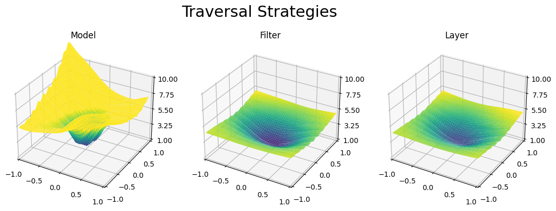
As seen above, we found that perturbation directions applied to the model as a whole were more reliable for evaluating vision transformers. In contrast, layer or filter perturbation techniques often reveal more information for highly structured models such as CNN’s.

Generation Metrics After determining a traversal strategy, determine how far to traverse and the density of points to plot. Larger model traversals capture broader information, relevant to the overall training efficiency and often revealing more information about the dataset. Smaller model traversals capture local changes, revealing more information about the optimization process and training progression.

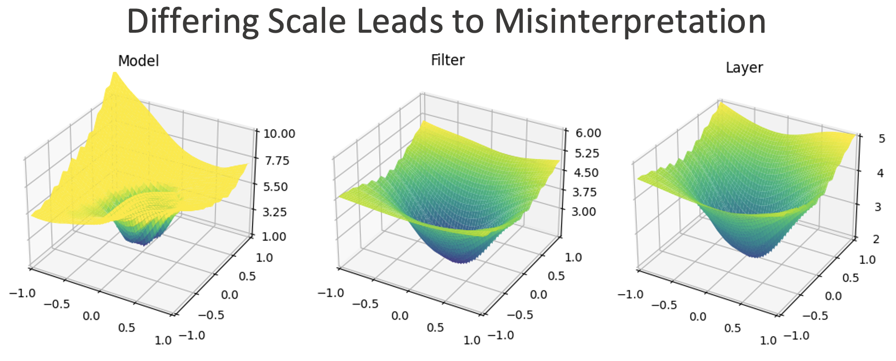
Plot Scaling and Coloring Last, plots must be graphed using the same scale and color gradients. Even slight differences in the coloring can lead to misleading comparisons. For example, if we were to replot the graph from Traversal Strategies, we could artificially scale the loss plot to find what seems to be a deeper or sharper landscape. Forgetting to scale all plots similarly make it difficult to gain insight from plots.

Loss Landscapes for Strategic Model Improvement

Small model hyperparameterization can quickly take place by training many models, but larger deep learning models often take significant compute. Thus, we propose using loss landscapes information early in training for strategic training plans. The first hyperparameter to tune is the learning rate. When training a Vision Transformer on various learning rates, we observed that smaller learning rates led the model to get stuck in local minima, while large learning rates prevent the model from converging. As seen in the plot below, the loss landscapes similarly reflect these observations.

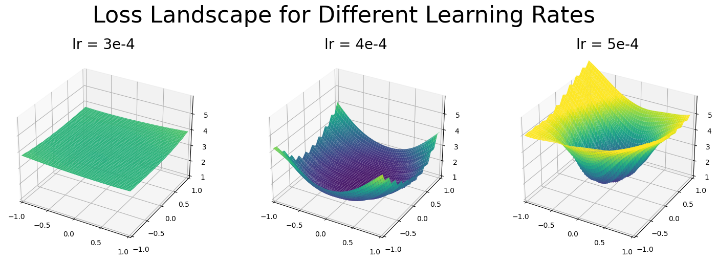
From these results, we can easily anticipate learning rates that are set too large, as the model fails to explore plausible paths and has a non-decreasing minima with a completely flat loss landscape. We can not easily anticipate when the learning rates are too small, as the above plot may not distinguish early convergence with a local minima with exploring a deep solution.

Thus, we analyzed how the plot landscape evolves throughout training with and without SAM. Below, we see that SAM explores the loss landscape with substantially more wide minima.

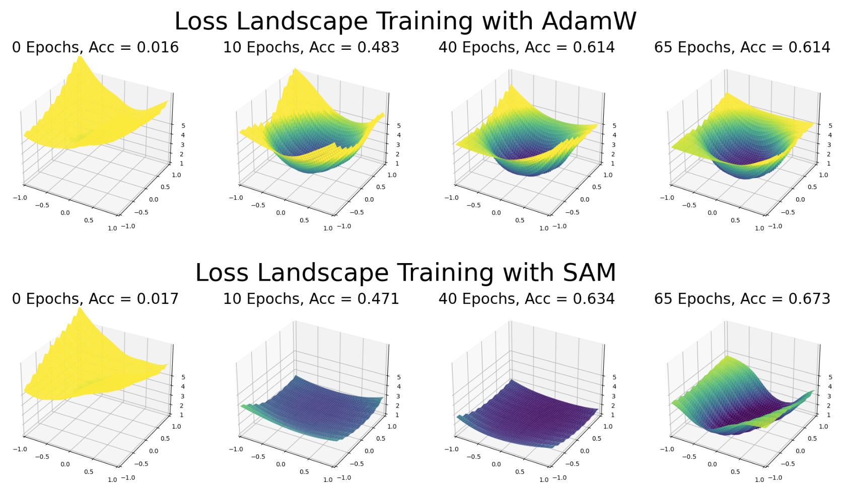
Additionally, the loss pattern of SAM can be distinguished from an improperly scaled training loss landscape with the base optimizer by the edge values. In the base optimizer, AdamW, the values return to the loss of a randomly initialized model (loss ~6). In SAM, the loss landscape is wide, and the edge loss values substantially decrease relative to the initial loss. Interestingly, it is not until the model is converging on a final solution that the loss for the edge conditions begin to increase. We speculate that this curling effect is due a sign of the model beginning to overfit the data.

Last, we found an interesting observation that small values of rho (the influence factor) with SAM still led to a remarkable improvement of the model over the base optimizer, but yet a substantially sharper loss landscape in the end. As seen below, SAM trained with rho = 1 had a much sharper loss landscape than the base optimizer.

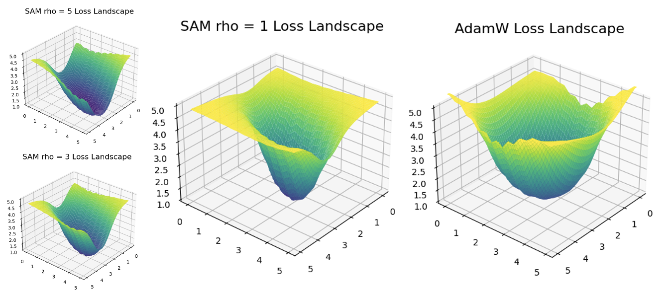
Furthermore, the test accuracy of the model trained with SAM rho = 1 was closer in performance to SAM trained with rho = 5, than it was to the base optimizer.

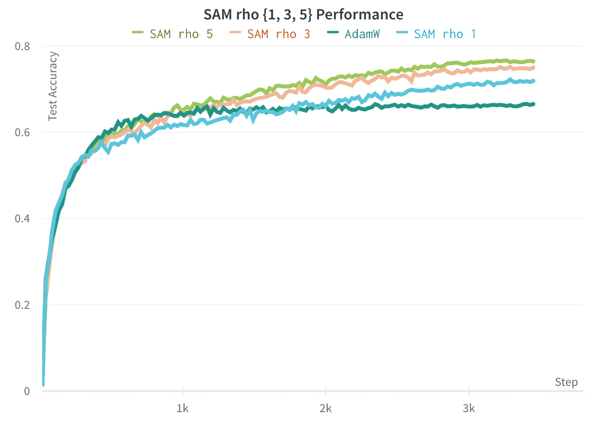
Thus, we see how the final final training landscape of a model does not tell the full story. We anticipate the most important use of loss analysis for large models will be in hyperparameter tuning and mid-training analysis. As larger models are being trained, expertise in the loss landscape will grow in importance. We hope this blog provides a great resource for understanding how to plot, interpolate, and use loss landscapes for improving model training.